Introduction to Data Compression

index

Introduction

Data flows everywhere, it is in every product that we interact with daily. More than 2.5 quintillion bytes are created every day (that is 2.5 followed by 18 zeros). For the next 5 years data is expected to grow by 40% every year.

We need, and will continue to need, more powerful and faster computers capable of processing this increasing amount of information, and better storage systems to safekeep it.

There has been a lot of improvement hardware-wise in the last couple of decades, which increased the density of our storage systems. However, what if we could improve our information storage density through other, non-physical, means? What if we could store the same amount of “information” but with fewer “bits”? This would allow us to work in parallel with scientists researching physical systems.

This is where data compression comes in. It allows us to store the same amount of “information” in less bits, digits, characters, or whatever the most basic unit of storage is in our medium of choice. An early example of compression work is the Morse Code, which was invented in 1838 for use in the telegraph industry. Telegraph bandwidth was scarce, so shorter code words were assigned for common letters in the English alphabet, such as “e” and “t”, that would be sent more often.

Compression can also be useful for analysis and recognition of data patterns. Suppose that given a telegraph system, we had decided to make a picture for every single letter in the English alphabet, and instead of sending Morse code over a telegraph, we had sent all the pixel information for the letter images every time we wanted to transmit a sentence across the wire. Not only would that have taken so much longer and wasted bandwidth (related to compression), but it would also have been way harder to recognize and would have been more error prone (people’s calligraphy is different from one another). One would have to record all the pixel information for every letter, reconstruct it, and then decide on which letter it is: a computationally hard and intensive task for both a computer and a human.

Morse code, an example of compression, shows how crucial it is to find reliable ways of storing and sharing our information in a way that minimizes space used and maximizes reliability.

Mathematical Background

There are various tools at our disposal that we can use to study and perform data compression and analysis. Many of the common techniques that are used today are the outcome of collaboration between scientists and engineers focused on different branches of Math, such as Probability, Statistics, Information Theory, and Linear Algebra.

While we have focused on Linear Algebra this semester, it is necessary to know some introductory concepts from these other branches to understand basic data compression. In this section we will introduce these branches and explain some of their basic concepts.

Probability & Statistics

Probability is the study of the likelihood of events, independently and given the occurrence of other events (e.g., given that it is cloudy, what is the probability that it will rain today?). Statistics is the discipline that concerns the collection, organization, analysis, interpretation, and presentation of data.

Sample Space

The most basic concept in probability is that of the sample space and events.

Definition (Sample Space)

The sample space is the set of all possible outcomes that an experiment can have.

Example (Flipping a coin)

If we flip a coin then the sample space is $S = \{\text{Heads}, \text{Tails}\}$ .

Example (Rolling a die)

If we roll a single 6-sided die the sample space is $S = \{1, 2, 3, 4, 5, 6\}$ .

Events

Definition (Event)

Events are mathematically defined as a subset of the sample space.

Example (Rolling a die)

For example, in the 6-sided die example let $M$ be the event we roll a 4 or greater. Then $M = \{4, 5, 6\} \subseteq S$ .

In this experiment we state that we are rolling the die once, so we cannot make any statements about what happens if you first roll something, and then something else. In that case, one would have to redefine the experiment to say that each die roll has possibilities $R = \{1, 2, 3, 4, 5, 6\}$ and the total experiment with $n$ rolls has sample space $S = R^n$ .

Probability

Definition (Probability)

The probability of an event (denoted $P(M)$ for an event $M$ ) is the measure of how likely the event is to occur as the outcome of a random experiment. It is the sum of the probabilities of each element of the set being the outcome of the performed experiment.

Probability is measured out of 1, which means that events certain to occur have a probability of 1 and events that will never occur have a probability of 0.

Since the sample space contains all the possible outcomes for the experiment, it is guaranteed that one of the sample space’s elements will be the outcome of the experiment, so $P(S) = 1$ .

Random Variables

Definition (Random Variables)

Random variables (also r.v.’s) are functions that map the outcome of a random experiment (in the sample space) to a measurable quantity (e.g., real number) or a mathematical object (e.g., matrix).

When the experiment is performed, and the outcome is mapped to a value, we say the random variable “crystallizes” to that value. The set of all values a random variable crystallizes to is called the support, denoted $R_X$ for a r.v. $X$ . A specified random variable crystallizing to a certain value is an event.

We normally denote random variables with capital letters and their crystallized values with lower case letters.

Example (Flipping a coin)

Let us flip a fair coin with equal probabilities of landing heads or tails. The sample space is then $S = \{H, T\}$ with $P(\{H\}) = P(\{T\}) = 0.5$ .

Let $X$ be a random variable that crystallizes to $-1$ if the coin lands Heads and to $1$ if the coin lands Tails. Then $(X = -1)$ and $(X = 1)$ are events and we write $P(X = -1) = P(\{H\})$ and $P(X = 1) = P(\{T\})$ .

If we were to write the probability function for $X$ , where $x$ is the crystallized value that $X$ takes, we would get:

P(X = x) = \begin{cases} 0.5 & \text{if } x = -1 \\ 0.5 & \text{if } x = 1 \end{cases}

Expectation

Definition (Expectation)

The expectation (also called the mean) of a random variable $X$ , denoted $\mathbb{E}(X)$ , is the weighted average of the values that $X$ can take. The weight for a value $x$ is determined by the probability of $X$ crystallizing to that value.

We also write the variable with a bar on top to represent its mean. Its formula is:

\bar{X} = \mathbb{E}(X) = \sum_{x \in R_X} x \cdot P(X = x)

Example (Rolling a die)

Expanding on the previous example of rolling a 6-sided die once. Let $X$ be a random variable that crystallizes to the number rolled. Then $R_X = \{1, 2, 3, 4, 5, 6\}$ and $P(X = x) = \frac{1}{6}$ for all $x \in R_X$ , since each number has the same probability of being rolled.

The expected value of $X$ is then:

\mathbb{E}(X) = \sum_{x \in R_X} x \cdot P(X = x) = \frac{1}{6} \cdot 1 + \frac{1}{6} \cdot 2 + \frac{1}{6} \cdot 3 + \frac{1}{6} \cdot 4 + \frac{1}{6} \cdot 5 + \frac{1}{6} \cdot 6 = \frac{21}{6} = 3.5

Variance

Definition (Variance)

Variance is a measure of spread. It measures how far the values in the support of an r.v. are from the mean. For a r.v. $X$ we denote its variance as $\text{Var}(X)$ . The formula for variance is:

\text{Var}(X) = \mathbb{E}[(X - \bar{X})^2] = \mathbb{E}(X^2) - [\mathbb{E}(X)]^2

Below is a graphical comparison between the probability function of a low variance r.v. $X$ and the probability function of a high variance r.v. $Y$ . The horizontal axis indicates a value in the support of the random variable and the vertical axis indicates the probability of the random variable taking that value.

Low variance distribution — Low Variance

High variance distribution — High Variance

Covariance

Definition (Covariance)

While the variance is the measure of spread for a single variable, the covariance examines the directional relationship between two variables. Its formula is:

\text{Cov}(X, Y) = \mathbb{E}[(X - \bar{X})(Y - \bar{Y})] = \mathbb{E}(X \cdot Y) - \mathbb{E}(X)\mathbb{E}(Y)

If greater values of one variable correspond to greater values of the other variable, covariance is positive. If greater values of one variable correspond to lesser values of the other variable, covariance is negative.

Below is a graphical comparison of what negative, zero, and positive covariance looks like between two random variables. Each point encodes one instance of the two variables crystallized together.

Negative covariance scatter plot — $\text{Cov}(X, Y) = 0$

Zero covariance scatter plot — $\text{Cov}(X, Y) = 0$

Positive covariance scatter plot — $\text{Cov}(X, Y) = 0$

If covariance is 0, we say that variables are “uncorrelated”, and we interpret it as there being no linear relationship between the two.

Start of the Story: What do we want to compress?

Handwriting Recognition

One of the oldest and most accessible methods of communication within a given language is writing by hand. Although in recent years there has been a large effort to make society paper-free, computers still process paper-based documents from all over the world every day in order to handle, retrieve, and store information. An efficiency problem arises, however, from the fact that it requires a lot of time and money to manually enter the data from these documents into computers. A solution to this efficiency problem is required, as these documents may continue to need processing for the foreseeable future due to a number of reasons, including historical record keeping. Up until recently, most of these were handwritten or on print paper. Examples include doctors’ prescriptions, government documents, and immigration papers.

Thus, handwriting recognition is the task of transcribing handwritten data into a digital format, and this task obviously benefits from data compression. The goal is to electronically process handwritten data, and to do so in a manner that achieves the same accuracy as humans.

Handwriting can essentially be categorized as either print or cursive script, and for both categories, recognition accuracy is the main problem because of the similar strokes and shapes of some letters. Factors such as illegibility of handwriting can yield inaccurate recognition of a letter by the software. Finally, a complicating problem that makes recognition notably difficult (especially for cursive) is the absence of obvious character boundaries; while print handwriting often has gaps and spaces between each letter, this is most often not the case for cursive writing, and so it is hard to know the start and stop of recognition per character.

This is where the data compression/dimension reduction and eigenface technique comes into play! In essence, if we have a large data set that consists of thousands or even millions of images of words (probably limited to one language), we want to find a way to recognize patterns in these images. From these patterns, we can then determine which ones have the most “importance” and attempt to express these images as a weighted combination of these most important patterns (and thus in a lower dimension).

Principal Component Analysis

Extracting “high information” regions in the data space

In this chapter we will see how we can use the knowledge from the previous sections to find efficient representations for arbitrary data, and apply that to the challenge of handwriting recognition.

Data in its raw or most simple representation is likely to have the potential to store many more values than we actually care about. For example, in the case of character recognition, let’s say that the dataset that we have for each handwritten character consists of 28×28 pixel grayscale images.

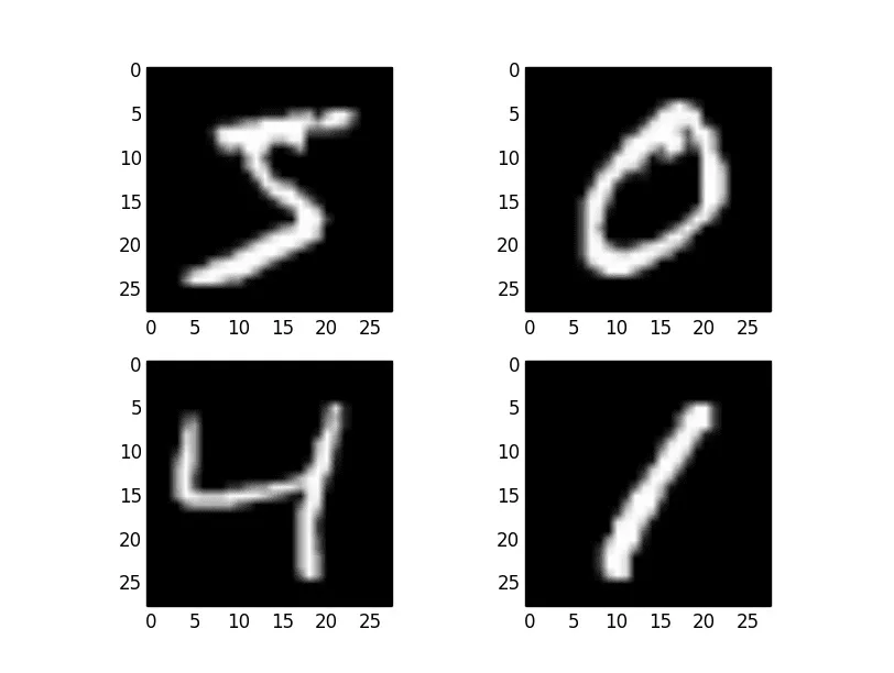
*Figure 1: Samples of the numbers 5, 0, 4, and 1 from the MNIST handwriting dataset.*

Theoretically, with this data space, we can encode significantly more than the letters and digits in the English alphabet. An all black or all white image exists in this data space but does not represent any of the glyphs that we care about.

The aim of data compression is to find a way of reducing the size of our data representation while preserving the ability to reconstruct the information in the original uncompressed data space at will.

In the case of the alphabet and humans, it is quite straightforward. A person can read a character, store it in the computer as a numerical value (0-9 for ‘0’-‘9’ and 10-35 for ‘a’-‘z’), and then when we want an image again, a human can write the digit out. But this technique is very restricted. It can only be applied to the characters the human is able to remember and that we had previously encoded as a numeric value. If the person sees a new digit they do not recognize, there is no way of storing this information using this compression format.

We need to establish a system that is able to solve this problem, that can be performed by computers without human intervention, and that can encode more than a predefined set of discrete values (ideally a continuous spectrum of variables).

A common technique that has these capabilities is called Principal Component Analysis (PCA). At a high level, it consists of finding patterns in the data (called components) and creating a system that allows us to express a datapoint in our original data space in terms of how much of each component appears in that point.

Example (Compressing images of plaid patterns)

In this example, we will look at a set of images that consists of plaid patterns and see how PCA can be useful in reducing the amount of data it takes to store these.

Four plaid pattern images — *Four sample plaid pattern images in an 8×8 pixel grid.*

The standard representation of this data would be a vector of $8 \times 8 = 64$ dimensions, where each dimension can take one of three values: 0 (black), 1 (gray) or 2 (white). This data space would have $3^{64} \approx 3.43 \cdot 10^{30}$ elements but most of them would not represent plaid patterns, which is what we know our data will always represent.

Note

To store one of these datapoints would require storing the pixel value for each dimension, resulting in a storage size of 128 storage units.

What if we expressed these datapoints in a more favorable basis? Let the following be our new basis for expressing datapoints:

16 basis vectors for plaid patterns — *A set of 16 basis vectors: 8 vertical stripe patterns and 8 horizontal stripe patterns.*

If we express our datapoints as a linear combination of these vectors, then we can recreate any of the images presented above, and any other plaid pattern that we want. Importantly, we represent any pattern by just 16 values, the coefficients for each basis vector.

With this basis, we can only represent $2^{16} = 65536$ datapoints, but those will be all the plaid pattern combinations that exist within the original dataspace. For example, we can obtain the four images above by taking the following linear combinations of the basis vectors:

Linear combinations showing how basis vectors combine to form plaid patterns — *Each plaid pattern can be expressed as a sum of horizontal and vertical stripe basis vectors.*

A linear algebra analogy

We can draw the analogy from the abstract high-level concepts that we just looked at to the change of basis procedures that we studied in class. As mentioned above, each datapoint is a vector, and an “expression system” is simply a set of basis vectors that can be used to write out datapoints in an expressed form.

By the theorem seen in class, if one has the same number of linearly independent vectors as dimensions in a space, that set of vectors forms a basis. But if we find a set of $n$ vectors to represent datapoints in an $n$ -dimensional space, we have achieved no compression, since we can use the standard basis and obtain the same storage efficiency.

Ideally the dataset that we want to represent only contains vectors in a lower-dimensional subspace of the data space. That way, we can express all the data points we are interested in with a smaller number of vectors.

Unfortunately, real world data rarely fits a proper mathematical subspace, so this technique would not be reliable for all types of data. For example, assume all our data is on a plane within a 3-dimensional data space. With just one point that is not within the plane, we have increased the dimension of our subspace to 3, yielding no compression when expressing datapoints with new eigenvectors.

Our method must take into account how “important” these areas of space are to decide whether it is worth reducing our compression efficiency to be able to represent only a few infrequent datapoints.

Formalizing the calculation of “high information” eigenvectors

How can we use the knowledge we gained from principal component analysis, along with our linear algebra skills, to derive an algorithm for object recognition?

The answer lies in a 1987 paper written by L. Sirovich and M. Kirby, followed by the work of Matthew A. Turk and Alex P. Pentland, mathematicians who invented the method of “eigenfaces”. One of the earliest face detection methods, eigenfaces use rather simple math to achieve remarkable data compression that allows for mathematical descriptions of low-dimensional images.

Let us walk through the process of creating eigenfaces and discover their utility. As we will see later, our method will generalize nicely to characterizing other detectable objects. We start with a training set of $M$ images of faces. The larger the training set, the greater the precision of the algorithm. Each image in the training set must have the same resolution. In this case we will take them to be $N \times N$ pixels ( $N$ height and $N$ width) without loss of generality. Our goal is to represent each face as a vector, and we do this by placing the $N$ columns into one single column vector of $N^2$ dimensions. Each pixel in this arrangement is a variable of 256 possible color values, and our image is called an 8-bit image (8-bit images are standard, however this process is independent of our choice of $N$ ).

Example (Low Resolution)

Consider an extremely low resolution $2 \times 2$ pixel image. We can represent this image as a $2 \times 2$ matrix $A$ , defined:

A = \begin{pmatrix} 1 & 64 \\ 32 & 143 \end{pmatrix}

Since each pixel has 256 possible values that define its color, each entry in $A$ has some value between 0 and 256. We now change $A$ into a four-dimensional vector $\vec{v}$ such that:

\vec{v} = \begin{pmatrix} 1 \\ 64 \\ 32 \\ 143 \end{pmatrix}

Notice that this operation does not change the information contained in each image, it simply gives us an object that is easier to work with. Doing this operation on each of our $M$ images, we can now refer to the $a^{th}$ face vector as $\Gamma_a$ , where $1 \leq a \leq M$ . Having defined our vectors, let us turn to principal component analysis.

The motivation for using principal component analysis is to find what mathematicians Turk and Pentland referred to as “face space.” The face vectors live in large dimensional spaces ( $65,536$ -dimensional space for a $256 \times 256$ image). The goal at this stage is to reduce our large input vector space to a lower dimensional subspace. We will do this by taking the eigenvectors of a covariance matrix. From there, we will be able to write any face as a linear combination of these eigenvectors.

In defining this matrix, let us revisit our definition of covariance and adapt it from a mathematically defined random variable to one comprised of samples.

Definition (Sample Covariance)

In order to construct the covariance matrix, we need to define covariance for samples of a random variable that holds some true distribution that we lack knowledge of.

Let $\sigma(X, Y)$ be the covariance between r.v.’s $X$ and $Y$ , and let $X_a$ be the $a^{th}$ sample of the $X$ random variable, and $\bar{X}$ the sample mean (weighted average value of r.v. based on number of appearances in dataset).

Mathematically, sample covariance is then defined as:

\sigma(X, Y) = \frac{1}{M} \sum_{a=1}^M (X_a - \bar{X})(Y_a - \bar{Y})

Definition (Covariance Matrix)

The covariance matrix is a matrix that measures the covariance between each pair of variables. We denote the variables as $x_1, \ldots, x_p$ . If we have $N^2$ variables, our covariance matrix is a $N^2 \times N^2$ matrix:

C = \begin{pmatrix} \sigma_{11} & \sigma_{12} & \cdots & \sigma_{1p} \\ \sigma_{21} & \sigma_{22} & & \\ \vdots & & \ddots & \\ \sigma_{p1} & & & \sigma_{pp} \end{pmatrix}

where the entry $\sigma_{ij}$ represents the covariance between the $i^{th}$ and $j^{th}$ variables.

In the case of eigenfaces, the $p$ variables correspond to each of the $N^2$ pixels in an image. Thus, $p = N^2$ for our application, where $N$ is the width and height of an image.

Having defined our covariance matrix, we must now discuss why we are taking the eigenvectors of this particular matrix to be our eigenfaces. The answer lies in the fact that the eigenvectors of the covariance matrix are the directions of maximum variance in the data. In other words, the eigenvectors of the covariance matrix are the directions of maximum information.

We calculate the eigenvectors so that we simplify a relation based on matrix multiplication to a relation defined by scalar multiplication, so that we may write any face as a linear combination of eigenvectors.

Taking an eigenvector $u$ , we have $Cu = \lambda_u u$ . Notice that if $\lambda_u$ is large, then the amount of information contained in the direction of $u$ is large. Thus, we can use the eigenvectors of the covariance matrix to represent our faces in a lower dimensional space by discarding the low eigenvalue ones and projecting all images to the subspace spanned by the remaining eigenvectors.

Eigenfaces are sometimes referred to as “ghost-like” images, given their slightly vague features. Intuitively, we can understand each eigenface as a sort of general face, where a greater eigenvalue implies a more general face. By combining general faces with more specific faces, we can obtain an approximation of any other face (that is reasonably similar to our training set).

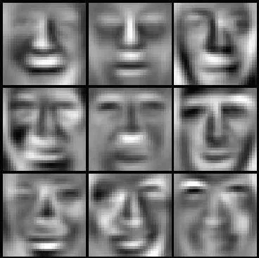
Ghost-like eigenfaces — *Figure 2: “Ghost-like” eigenfaces.*

Before we discuss the eigenvalues, however, we must derive some more properties of $C$ that will ultimately help us condense our data.

Firstly, given the large size of $N^2$ , it is convenient for us to find a more condensed description of the covariance matrix.

Theorem (Simplified Covariance Matrix)

Let $C$ be a $p \times p$ covariance matrix where each matrix entry $c_{ij} = \sigma_{ij}$ . Define the variance:

\Phi_a = P_a - \bar{P}

where:

P_a = \begin{pmatrix} x_{1a} \\ x_{2a} \\ \vdots \\ x_{pa} \end{pmatrix}, \quad 1 \leq a \leq M

Then, the covariance matrix can be written as:

C = \frac{1}{M} \sum_{a=1}^M \Phi_a \Phi_a^T

Proof

We can start the proof of this theorem with our matrix:

C = \begin{pmatrix} \sigma_{11} & \sigma_{12} & \cdots & \sigma_{1p} \\ \sigma_{21} & \sigma_{22} & & \\ \vdots & & \ddots & \\ \sigma_{p1} & & & \sigma_{pp} \end{pmatrix}

For any entry, $c_{ij} = \sigma_{ij}$ . From the definition of covariances, each entry:

c_{ij} = \frac{1}{M} \sum_{a=1}^M (x_{ia} - \bar{x}_i)(x_{ja} - \bar{x}_j)

Since matrices add linearly, we can factor out the summation $\frac{1}{M} \sum_{a=1}^M$ . Now we can write the whole matrix:

C = \frac{1}{M} \sum_{a=1}^M \begin{pmatrix} (x_{1a} - \bar{x}_1)(x_{1a} - \bar{x}_1) & \cdots & (x_{1a} - \bar{x}_1)(x_{pa} - \bar{x}_p) \\ \vdots & \ddots & \\ (x_{pa} - \bar{x}_p)(x_{1a} - \bar{x}_1) & & (x_{pa} - \bar{x}_p)(x_{pa} - \bar{x}_p) \end{pmatrix}

Now consider the term $\Phi_a \Phi_a^T = (P_a - \bar{P})(P_a - \bar{P})^T$ , as defined in the theorem. Since the transpose operator is distributive:

(P_a - \bar{P})(P_a - \bar{P})^T = \begin{pmatrix} x_{1a} \\ x_{2a} \\ \vdots \\ x_{pa} \end{pmatrix} - \begin{pmatrix} \bar{x}_1 \\ \bar{x}_2 \\ \vdots \\ \bar{x}_p \end{pmatrix}) \cdot (\begin{pmatrix} x_{1a} & x_{2a} & \cdots & x_{pa} \end{pmatrix} - \begin{pmatrix} \bar{x}_1 & \bar{x}_2 & \cdots & \bar{x}_p \end{pmatrix})

= \begin{pmatrix} x_{1a} - \bar{x}_1 \\ x_{2a} - \bar{x}_2 \\ \vdots \\ x_{pa} - \bar{x}_p \end{pmatrix} \begin{pmatrix} x_{1a} - \bar{x}_1 & x_{2a} - \bar{x}_2 & \cdots & x_{pa} - \bar{x}_p \end{pmatrix}

Multiplying these two matrices, we get:

\Phi_a \Phi_a^T = \begin{pmatrix} (x_{1a} - \bar{x}_1)(x_{1a} - \bar{x}_1) & \cdots & (x_{1a} - \bar{x}_1)(x_{pa} - \bar{x}_p) \\ \vdots & \ddots & \\ (x_{pa} - \bar{x}_p)(x_{1a} - \bar{x}_1) & & (x_{pa} - \bar{x}_p)(x_{pa} - \bar{x}_p) \end{pmatrix}

Notice that any entry $A_{ij}$ in this final matrix resembles the formula for the covariance between the $i^{th}$ and $j^{th}$ variable. The only component missing is the summation on all values of $a$ . Thus we can write:

C = \frac{1}{M} \sum_{a=1}^M \Phi_a \Phi_a^T

Recall that each vector has $N^2$ dimensions, corresponding to pixels, and that our training set has $M$ vectors. The first index $p$ marks the $p^{th}$ pixel, and the second index $a$ marks the $a^{th}$ image in the training set.

In the eigenface case, we wish to measure the difference between the face vectors $\Gamma_a$ and the average face. We define the average face $\bar{\Gamma}$ as follows:

\bar{\Gamma} = \frac{1}{M} \sum_{a=1}^M \Gamma_a

We can write the difference $\Phi_a$ between the average face and the $a^{th}$ face:

\Phi_a = \Gamma_a - \bar{\Gamma}

Following the rules of matrix multiplication, we can also rewrite our definition:

C = \frac{1}{M} \sum_{a=1}^M \Phi_a \Phi_a^T = AA^T

where $A$ is a matrix with columns $\begin{pmatrix} \Phi_1 & \Phi_2 & \cdots & \Phi_M \end{pmatrix}$ .

Now we express the eigenvectors $u_i$ and eigenvalues $\lambda_i$ of our covariance matrix as:

\lambda_i u_i = AA^T u_i

However, $AA^T$ is an $N^2 \times N^2$ matrix, which for images of any reasonable size is going to be very large.

Consider instead the eigenvalues of $A^T A$ :

A^T A v_i = \lambda_i v_i

Multiplying both sides of our equation by $A$ we get:

AA^T A v_i = \lambda_i A v_i

Therefore, for any eigenvector $v_i$ of $A^T A$ , $u_i = A v_i$ is an eigenvector of $AA^T$ .

We can now focus on the eigenvectors of $A^T A$ instead. The advantage of effectively reordering the $A$ and $A^T$ is that our new matrix is an $M \times M$ matrix. $M$ corresponds to the number of images in the training set, which in most cases is much smaller than the dimension of the resolution of the image. Therefore we have overcome the main obstacle in our path, and from this point on it will be much easier to compute the eigenfaces.

We can write each face in the training set as a linear combination of our $M$ eigenfaces:

\Gamma_a = c_{a1} u_1 + c_{a2} u_2 + \cdots + c_{an} u_n = \sum_{i=1}^M c_{in} u_n

Similarly, we can describe a face image not in the training set as a combination of weights and eigenvectors, by solving the above equation for the weights $c_{a1}, \ldots, c_{an}$ . We then compare its weights to the weights of “known” faces and evaluate whether it matches the weights of any of these faces to a certain degree of error. With this last step we have a complete picture of the facial recognition process.

We have walked through this process looking for facial recognition capabilities, as was the route taken historically, but this use of eigenvectors is actually much more general. We can apply this method to a variety of data recognition processes, including the others mentioned in this report.

Fingerprints, for example, are a very common form of biometric identification. The process of identifying a fingerprint is very similar to the facial recognition process.

With fingerprints, images are usually black or white (no gray), so we go from an 8-bit image to a binary 1-bit image. From there, we follow the same process as we did with facial recognition. We can use eigenvectors to represent “general fingerprints”, and we can identify new fingerprints by the weights it takes to represent them as a linear combination of eigenvectors. These “eigen-fingerprints” can be used in the same way as the eigenfaces to recognize fingerprints.

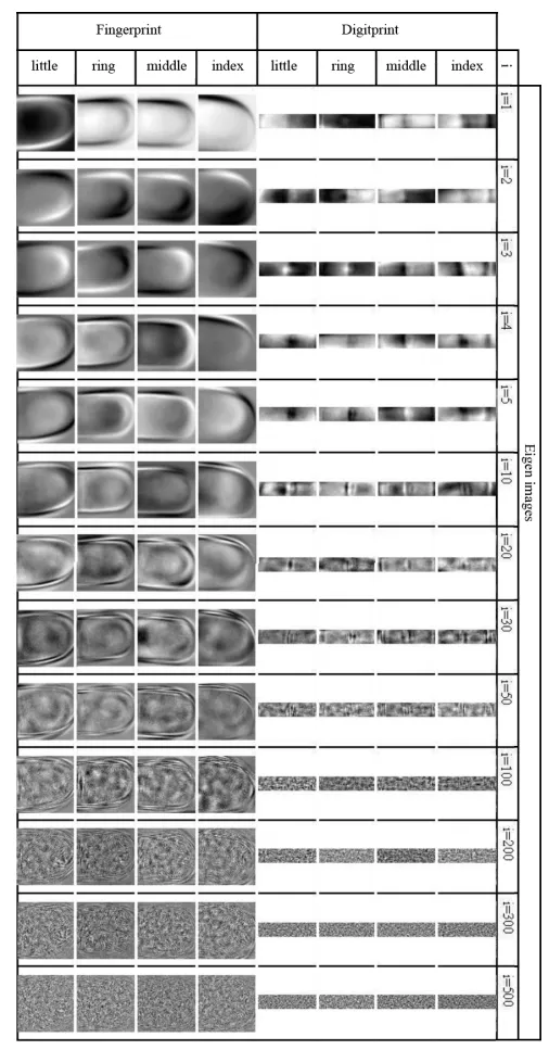
*Figure 3: Example eigen-fingerprints and eigen-digitprints; digitprints are simply another form of fingerprint image.*

Notice how these eigen-fingerprints get more detailed and granular as we increase the eigenvalue (in the image higher eigenvalues correspond with lower values of $i$ ). By combining these eigenvectors, we can recreate any reasonably similar fingerprint. This technology has direct applications in security, where a scanned fingerprint can be projected onto the subspace spanned by the chosen eigenvectors (typically less than the dimension of the original fingerprint image) and compared to a list of weights in the database of approved fingerprints. If the weights are very similar (less than a certain threshold of difference) with a fingerprint in the database, then access is granted.

Uses Beyond Compression

We mainly discussed how PCA allows us to reduce the dimensions of our data space and store data more efficiently, but there are more uses for this beyond compression. Having a simpler representation for our data allows us to perform more complex operations on it.

Classification

We can use PCA to perform classification on our data. After we have chosen our eigenvectors based on our initial dataset, and have manually classified the original “training” data into categories, we can use Linear Classification to classify new data into the preexisting categories.

This process consists of projecting the new datapoint to our lower-dimension subspace and then making a category decision based on how much weight each basis vector has in the new datapoint.

Recognition

In cases where there are no discrete categories defined during training time, we can use dimensionality reduction to more easily (and faster) compare a new datapoint to a list of known datapoints that continually gets updated.

In the case of facial recognition, we can use PCA to reduce the dimensionality of our data and then use a distance metric to compare the new datapoint to the known datapoints. The datapoint with the smallest distance to the new datapoint is the most similar and is therefore the most likely to be the same person.

References

Alexandra Q. (2015). Data Never Sleeps 3.0. Domo.
Marr, B. (2022). How Much Data Do We Create Every Day? Forbes.
Wolfram, S. (2002). A New Kind of Science. Wolfram Media.
Wikipedia contributors. Statistics. Wikipedia, The Free Encyclopedia.
Rice, J.A. (2007). Mathematical Statistics and Data Analysis (3rd ed.). Thomson Brooks/Cole.
Bortolozzi, F., et al. (2005). Recent Advances in Handwriting Recognition. Document Analysis.
Günter, S., & Bunke, H. (2005). Off-line Handwriting Recognition. In Handbook of Pattern Recognition and Computer Vision.
Holzinger, A. (2012). Human-Computer Interaction and Knowledge Discovery. Springer.
Puigcerver, J. (2017). Are Multidimensional Recurrent Layers Really Necessary for Handwritten Text Recognition? ICDAR.
Turk, M.A., & Pentland, A.P. (1991). Eigenfaces for Recognition. Journal of Cognitive Neuroscience, 3(1), 71-86.
Janakiev, N. (2018). Understanding Principal Component Analysis.
Dusenberry, M. (2015). Eigenfaces.
Wikipedia contributors. Eigenface. Wikipedia, The Free Encyclopedia.
Pavešić, N., et al. (2022). Fingerprint Recognition Using Eigenfingerprints.
Milon, M.H. (2019). Linear Classification Methods.