Introduction
Reinforcement Learning (RL) has undergone significant advancements, particularly within the realm of gaming scenarios, where agents grapple with the complexities of dynamic environments. While the landscape of RL literature has predominantly centered around scenarios framed by cooperation or competition, we explore intersection of RL and classic game theory, particularly the dynamics of multi-agent environments such as Iterated Prisoners’ Dilemma (IPD) and Chicken, where cooperation and competition is not fixed but dynamically unfolds.
We leverage Deep Q-Learning (DQN) to train our DQN agent in repeated games with 500-stage games per episode, and we vary the agents’ discount factor () and memory length (). Our DQN agent demonstrates the capacity to learn optimal strategies against TFT and Random, showcasing its ability to navigate single-agent environments. However, when pitted against other DQN agents, convergence tends towards a consistent (Defect, Defect) action profile in nearly every stage game.
Beyond the challenges encountered in Iterated Prisoner’s Dilemma (IPD), our investigation extends into the game of Chicken. We examine whether our DQN agents can learn to “signal” each other despite the use of independent Q-networks, potentially converging to correlated equilibria.
We made our modularized code for running future experiments publicly available and hosted on GitHub. It consists of an environment that can simulate a variety of normal form games and implementations for DQN, Random and TfT agents.
Reinforcement Learning
In reinforcement learning problems, agents map game states to actions to maximize a reward signal given by the learner’s environment. That is, at each time step , the agent receives an embedding of the environment state and selects an action . The agent then receives a reward and observes a new state, .
We can thus define single-agent Markov decision games as a tuple , where and are the sets of states and actions respectively, gives the probability of moving from one state to another after performing an action, and gives the expected reward for a state-action pair. The purpose of the agent is to maximize the total amount of reward it receives, that is , where is the discount rate, specifying the present value of future rewards.
We are interested in the class of multi-agent reinforcement learning (MARL). Shoham et al. extended the single-agent Markov decision games as follows:
Definition (multi-agent stochastic game): A multi-agent stochastic game can be represented as a tuple , where:
- is a set of agents indexed
- is a set of -agent stage games
- with the set of actions for player defined as
- with defining the immediate reward function of agent for the action taken in stage game
- is a transition function defining the probability of the next stage game to be played based on the previous stage game and the action profile played in it.
Q-learning
The basic idea behind Q-learning is to estimate the Q function by iteratively playing the game and updating values of state-action pairs. The value is defined to be the expected discounted sum of future payoffs obtained by taking action from state and following a policy that maximizes the reward after that.
That is, we first initialize our action-value function to arbitrary numbers. The algorithm starts this initial Q-value, and through exploration and exploitation, it learns to optimize its policy over time. From the current state , we select an action , which gives some immediate reward and brings the agents to the next state . We then use the Bellman equation:
to iteratively update , where and are the learning rates and discount factors, respectively. Theoretically, this algorithm is guaranteed to converge to , the optimal action-value function, with probability 1 if the environment is stationary and Markovian, i.e. if state-transition probabilities only depend on the current state and the action taken in it.
Deep Q-learning
Because of the immense number of possible states in realistic scenarios, Q-Learning algorithms were historically constrained to either simple environments or required supplementary information about the environment’s dynamics for effective implementation. The traditional Q-Learning approach is impractical in practice because our function is estimated for each sequence of states.
However, one can extend Q-Learning to the Deep Q-Network (DQN) method, which combines a convolutional neural network for feature representation with Q-learning training. Instead of using a table to store Q-values for each state-action pair, DQN uses a deep neural network to approximate the Q-function. The neural network takes the state as input and outputs Q-values for all possible actions, which allows it to handle high-dimensional state spaces and generalize learning across similar states.
In 2013, Google DeepMind applied reinforcement learning to very high-dimensional input, producing the first deep learning model to successfully learn policies for Atari video games. Instead of computing , an approximation was used to estimate the function, with . In previous literature, the function approximator was typically linear, but a neural network function approximator with weights was applied as a Q-network. The network was trained with stochastic gradient descent to minimize a sequence of loss functions that change at each iteration.
Furthermore, the authors introduced the concept of experience replay, a mechanism to store and randomly sample past experiences from a replay buffer during training.
Definition (Experience replay): Agent experiences at each time-step, in a dataset , are stored and pooled over many episodes into a replay memory with capacity . During the inner loop of the DQN algorithm, minibatch updates are sampled from , i.e. samples are drawn at random from the pool of stored samples. Then, the agent selects and executes an action according to an -greedy policy.
This not only allowed for each step of experience to be used in multiple updates, but also helped break the temporal correlation in the data. The full algorithm, with representing the embeddings of histories, is then as follows:
# Initialize replay memory D with capacity N# Initialize action-value function Q with random weights
for episode in range(1, M + 1): # Initialize sequence s_1 = {x_1} and preprocessed sequence φ_1 = φ(s_1)
for t in range(1, T + 1): # With probability ε select a random action a_t # otherwise select a_t = argmax_a Q*(φ(s_t), a; θ)
# Set s_{t+1} = s_t, a_t, x_{t+1} and preprocess φ_{t+1} = φ(s_{t+1}) # Store transition (φ_t, a_t, r_t, φ_{t+1}) in D # Sample random minibatch of transitions (φ_j, a_j, r_j, φ_{j+1}) from D
if phi_j_plus_1_is_terminal: y_j = r_j else: y_j = r_j + gamma * max_a_prime(Q(phi_j_plus_1, a_prime; theta))
# Perform gradient descent step on (y_j - Q(φ_j, a_j; θ))²The DQN algorithm achieved performance exceeding that of expert human players in several Atari games, showcasing its ability to learn effective strategies and adapt to different game dynamics. Furthermore, the researchers demonstrated that the DQN architecture and hyperparameters could be used across multiple Atari 2600 games without game-specific modifications. This highlighted the ability of DQN to generalize learning across diverse environments.
Deep Q-Learning in Multiagent Environments
However, in an environment with multiple agents, the theoretical guarantee of convergence does not apply because the environment is nonstationary as other agents learn and adapt their strategies. The environment state transitions and rewards are not only affected by the action of one agent, but the joint action of all agents.
To address the problem of Q-learning in multiagent environments, Tampuu et al. introduce independent deep Q-learning, which runs DQN for each agent under the assumption that everything else that occurs in the environment is passive. That is, the environment is the sole source of interaction between agents, so the agent does not operate under the assumption that there are other agents with their own policy acting.
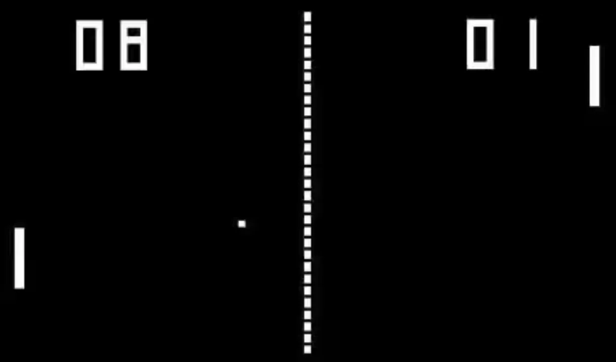 Figure 1: The Pong game.
The authors explore this under the Atari game Pong, modifying the rewarding schemes to induce cooperative or competitive behavior in their agents. The conventional reward system of Pong is competitive, where a player receives a positive point if they were the last to touch the outgoing ball, while the player conceding the ball incurs a negative point. This renders it a zero-sum game, wherein a gain in reward for one player corresponds to a loss for the other, and vice versa. The objective is to outscore the opponent by placing the ball behind them.
On the other hand, cooperative behavior is observed with a reward scheme that penalizes both agents when the ball goes out of play, regardless of who made the mistake. The scheme thus effectively rewards agents for learning to keep the ball in the game for as long as possible.
| Reward Scheme | Left scores | Right scores |
|---|---|---|
| Competitive / Classical (L,R) | 1, -1 | -1, 1 |
| Cooperative (L,R) | -1, -1 | -1, -1 |
| Transition (L,R) | ρ, -1 | -1, ρ |
Table 1: Reward schemes explored. Agents under the competitive reward scheme learn to score against their opponent efficiently, while agents under the collaborative reward scheme learn to keep the ball in the game (average paddle-bounces per point increases to ≈600, compared to between 3-10 in the noncooperative schemes). Agents did not swap from noncooperative to cooperative until ρ ≤ -0.75.
The authors thus demonstrate that independent deep Q-Networks can be used to study the decentralized learning of multiagent systems.
Prisoners’ Dilemma
Much of the literature similarly investigates games where agents have strong positively correlated payoffs (cooperation problems) or strong negatively correlated payoffs (competitive, zero-sum games). However, we aim to extend this framework to multiagent games where agents’ cooperation is not as defined by a reward function as in Pong. We thus turn to studying RL in Iterated Prisoners’ Dilemma (IPD), where agent payoffs are not strongly positively correlated nor strongly negatively correlated.
The Game
We’ll assume the payoffs for prisoners’ dilemma are the following:
| C | D | |
|---|---|---|
| C | 3, 3 | 0, 5 |
| D | 5, 0 | 1, 1 |
Note that if the number of stage games is known, then defecting on the last round is a dominant strategy, and inductively, defecting in the penultimate round is also a dominant strategy. As a result, agents are never motivated to cooperate throughout the sequence; hence we assume that the number of repetitions is not known, i.e. agents play as if they are playing infinitely-repeated Prisoners’ Dilemma.
The goal of the agent at stage game is thus to select actions that will maximize its discounted return:
where is the reward received in the th stage game and is the discount factor.
Experimental Setup
We train our DQN agent on 500 stage games per episode, varying and , our memory length. We will test our Q-Learning agents on the following known strategies:
- TFT: play C in round 1, then repeat the action that the other player took in the previous round
- Random: play C with probability 0.5 in each round
- Pavlov: play C in round 1. For subsequent rounds, if both agents cooperate in the previous round, play C with probability 1. If both agents defect in the previous round, play C with probability 0.95. Otherwise, defect.
We find Pavlov interesting to study because it can exploit Always Cooperate (if it defects by accident, it will keep greedily defecting, while Tit-For-Tat will not) but still exerts some pressure against Always Defect (defecting against it approximately half the time, compared to Tit-For-Tat’s consistent defection). Pavlov can beat TFT in a variety of scenarios because it fares better at cooperating than TFT if there is some randomness, which we might expect as our DQN agent explores initially. Furthermore, it concedes when punished, cooperating after (D,D) is played; hence we are interested in the optimal strategy against Pavlov.
We note that playing against these strategies is analogous to learning in a single agent environment because the opponent does not change its Q-values (i.e. opponent does not learn).
We are interested in how adaptive behavior arises over multiple rounds of the game. According to the Nash-Threat Folk theorem, for enforceable action profile in stage game , there exists a strategy profile and some discount factor such that is an SPE of for all discount factors and where action profile is played in every period on the equilibrium path. That is, the threat of noncooperative behavior serves as a mechanism to sustain cooperation and achieve outcomes that would not be possible in a one-shot game.
Because of this it is known that the optimal strategy against TFT is:
- If , always cooperate.
- If , alternate between defect and cooperate.
- If , always defect.
Hence, we can check to see if our DQN agent successfully learns these strategies given some discount factor.
IPD Results
DQN vs. Tit-For-Tat
We find that our deep Q-learning agent is able to learn the optimal strategy for all discount factors against TFT:
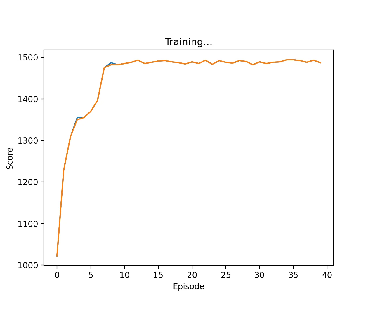 Figure 2: DQN Agent playing against TFT with a high discount factor (0.95) and memory length 5. The agent learns to cooperate on every stage game, approaching the score of 1500.
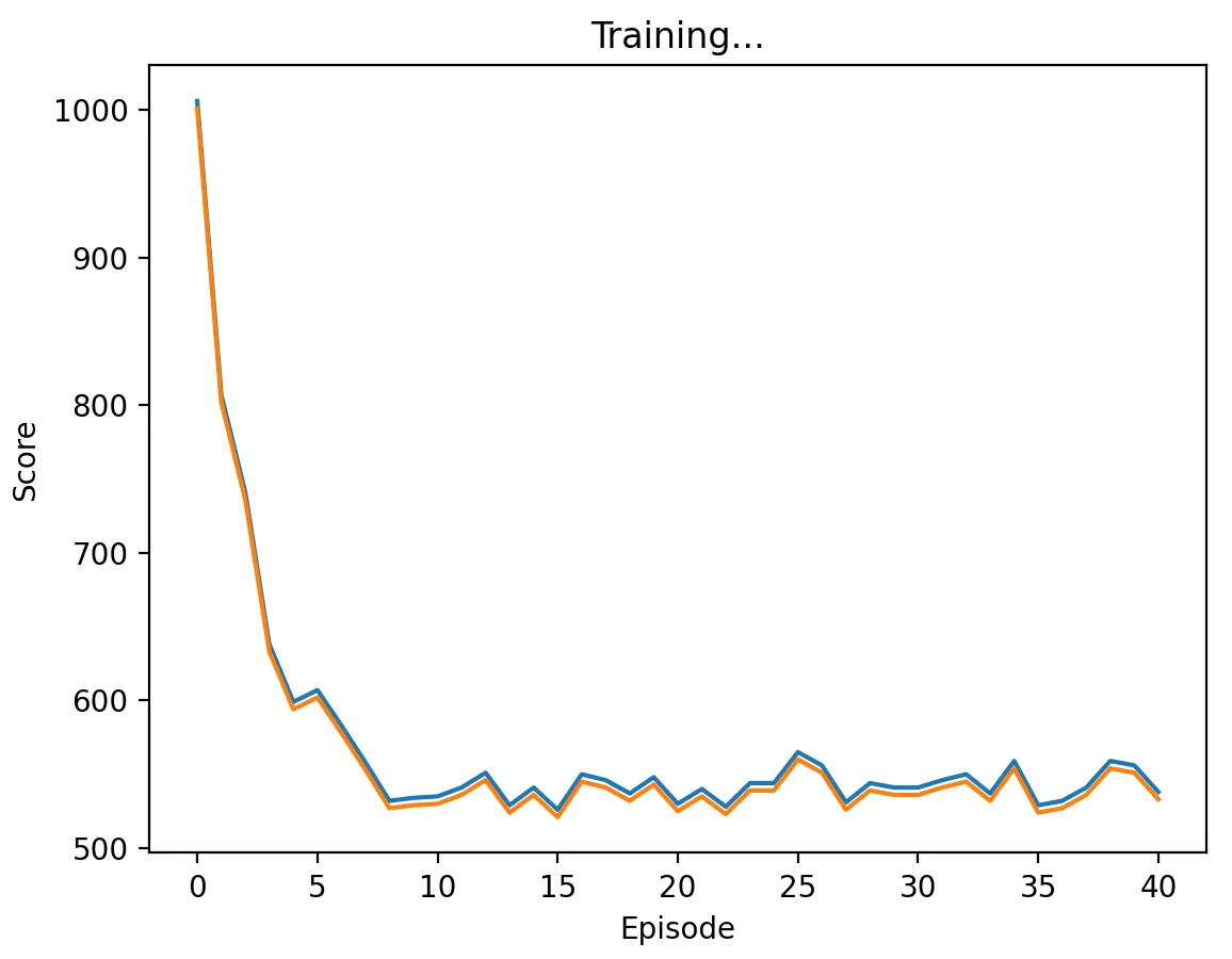 Figure 3: DQN Agent playing against TFT with a low discount factor (0.1) and memory length 5. The agent learns to defect on every stage game, approaching the score of 500.
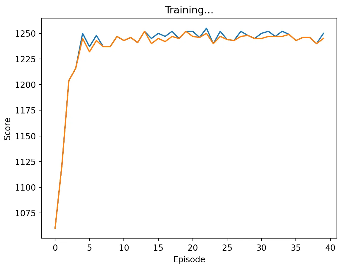 Figure 4: DQN Agent playing against TFT with a medium discount factor (0.5) and memory length 5. The agent learns to alternate between cooperate and defect on every stage game, approaching the score of 1250.
DQN vs. Random
With high, medium, and low discount factors, DQN quickly learns to defect at every stage game. Since the expected value of defecting in a given round against a random player is , we see the total score of our DQN agent in each episode converging to 1500. By the same logic, the expected score in a given round playing randomly against a player that always defects is , and we can see our Random agent quickly converging to a score of 250 per episode. As the discount factor decreases, our DQN agent defects more quickly; hence we see its score converging to 1500 faster as we decrease .
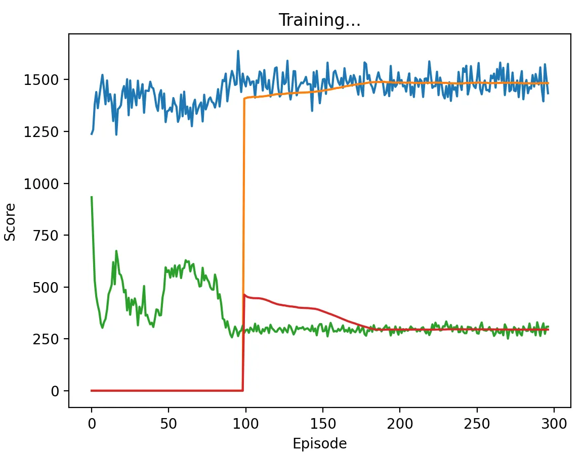 Figure 5: DQN Agent playing against Random with a high discount factor (0.95) and memory length 5. The agent learns to defect at every stage game, taking about 100 episodes to converge to a score of 1500.
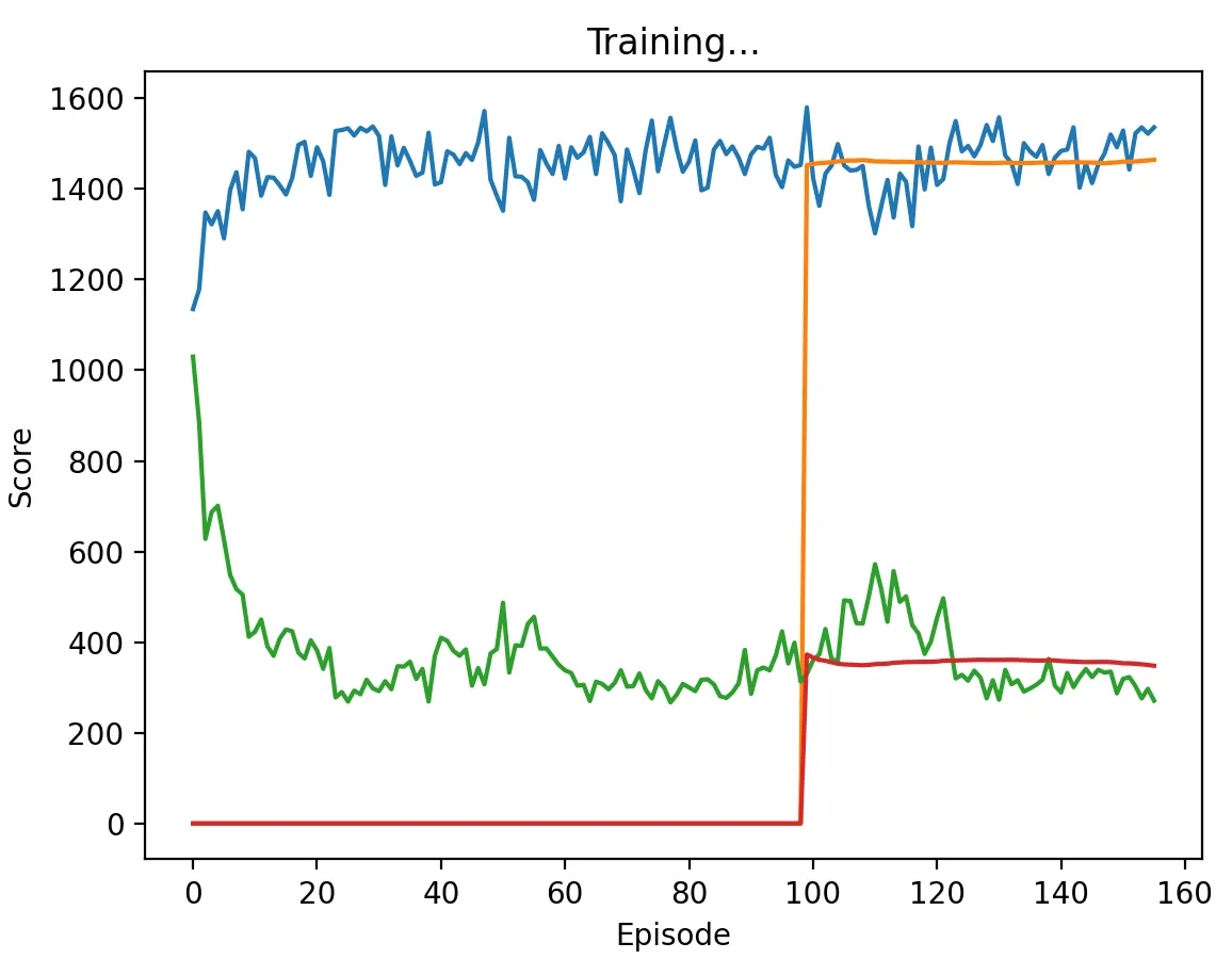 Figure 6: DQN Agent playing against Random with a low discount factor (0.1) and memory length 5. The agent learns to defect at every stage game, taking about 10 episodes to converge to a score of 1500.
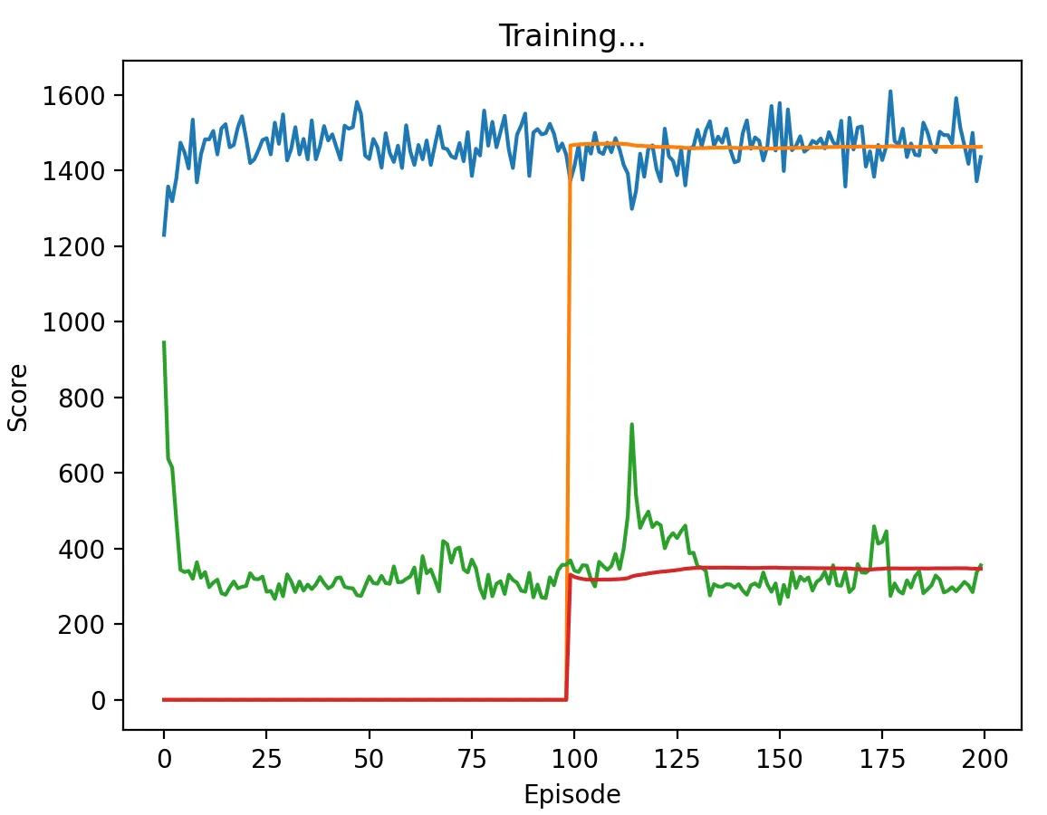 Figure 7: DQN Agent playing against Random with a medium discount factor (0.5) and memory length 5. The agent learns to defect at every stage game, taking about 15 episodes to converge to a score of 1500.
DQN vs. Pavlov
With high, medium, and low discount factors, DQN learns to outperform Pavlov relatively quickly, scoring about 50 points more per episode. We find that as the discount factor increases, DQN scores higher, likely because it is optimizing for cooperation in future rounds. However, unlike TFT, Pavlov takes advantage of always cooperate, so we see that the agent mixes defect into its strategy and is therefore unable to reach the same score as with TFT.
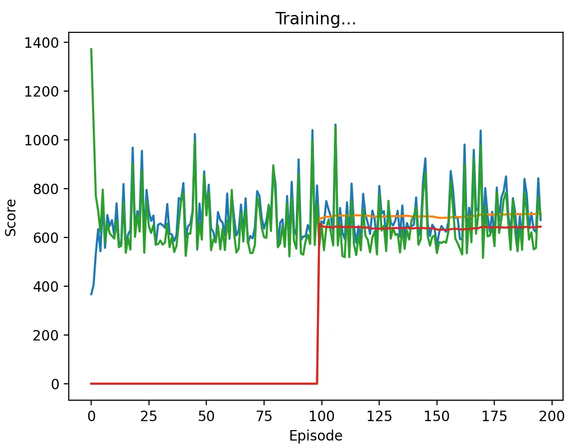 Figure 8: DQN Agent playing against Pavlov with a high discount factor (0.95) and memory length 5. The agent learns to cooperate on some of the stage games, approaching the score of 700. We note that this setting produced the highest variance in the DQN vs Pavlov experiments.
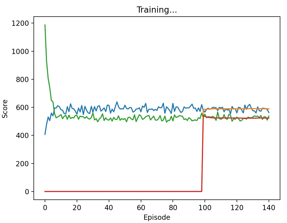 Figure 9: DQN Agent playing against Pavlov with a low discount factor (0.1) and memory length 5. The agent learns to defect on every stage game, approaching the score of 500.
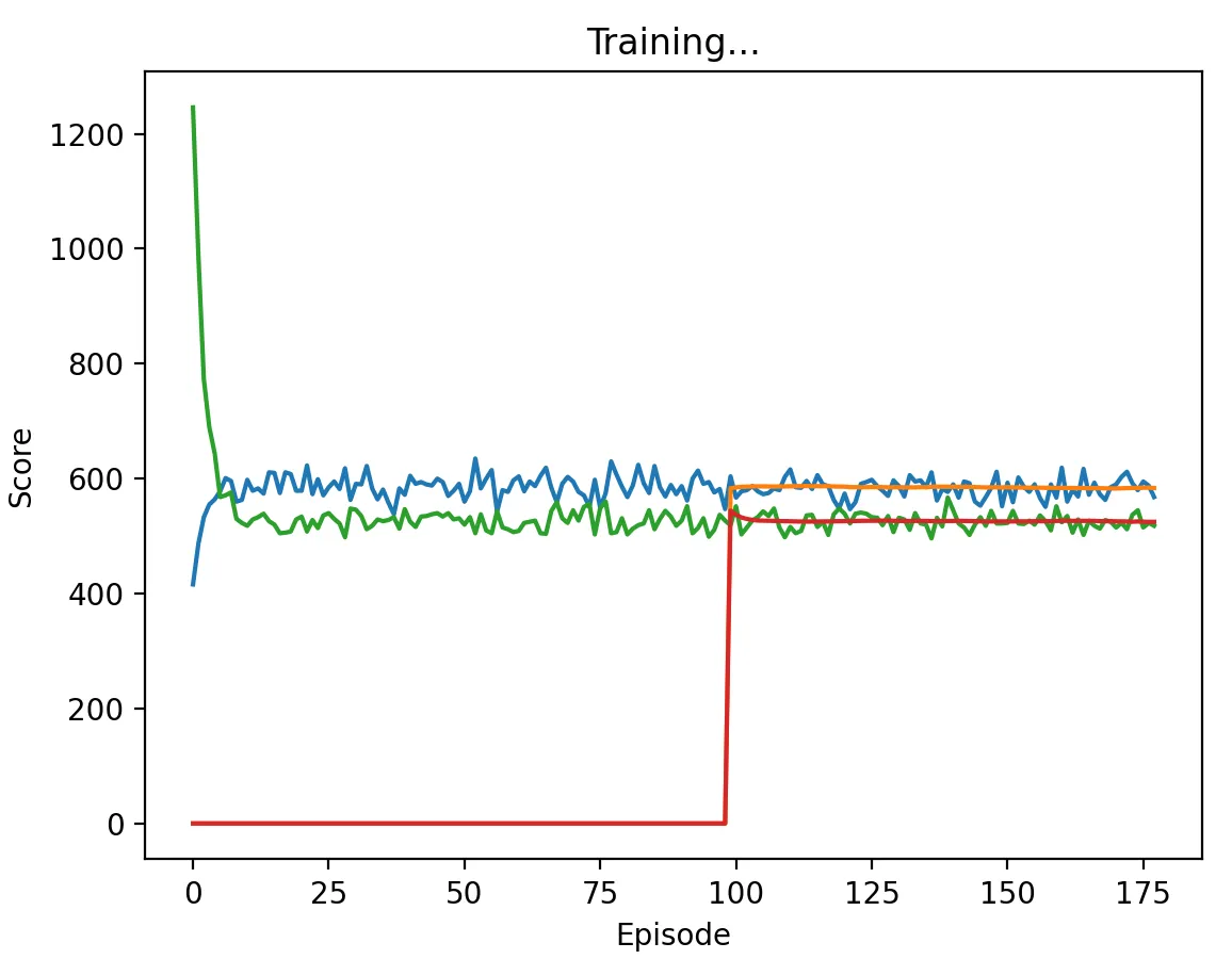 Figure 10: DQN Agent playing against Pavlov with a medium discount factor (0.5) and memory length 5. The agent learns to alternate between cooperate and defect on every stage game, approaching the score of 600.
DQN vs. DQN
As shown by the number of episodes it took to converge compared to playing against TFT, DQN agents had more difficulty playing against each other because the adaptation of the other agent created a nonstationary environment. Learners do not develop a model about the IPD game, so they learn without knowledge of any policy designed to encourage cooperation.
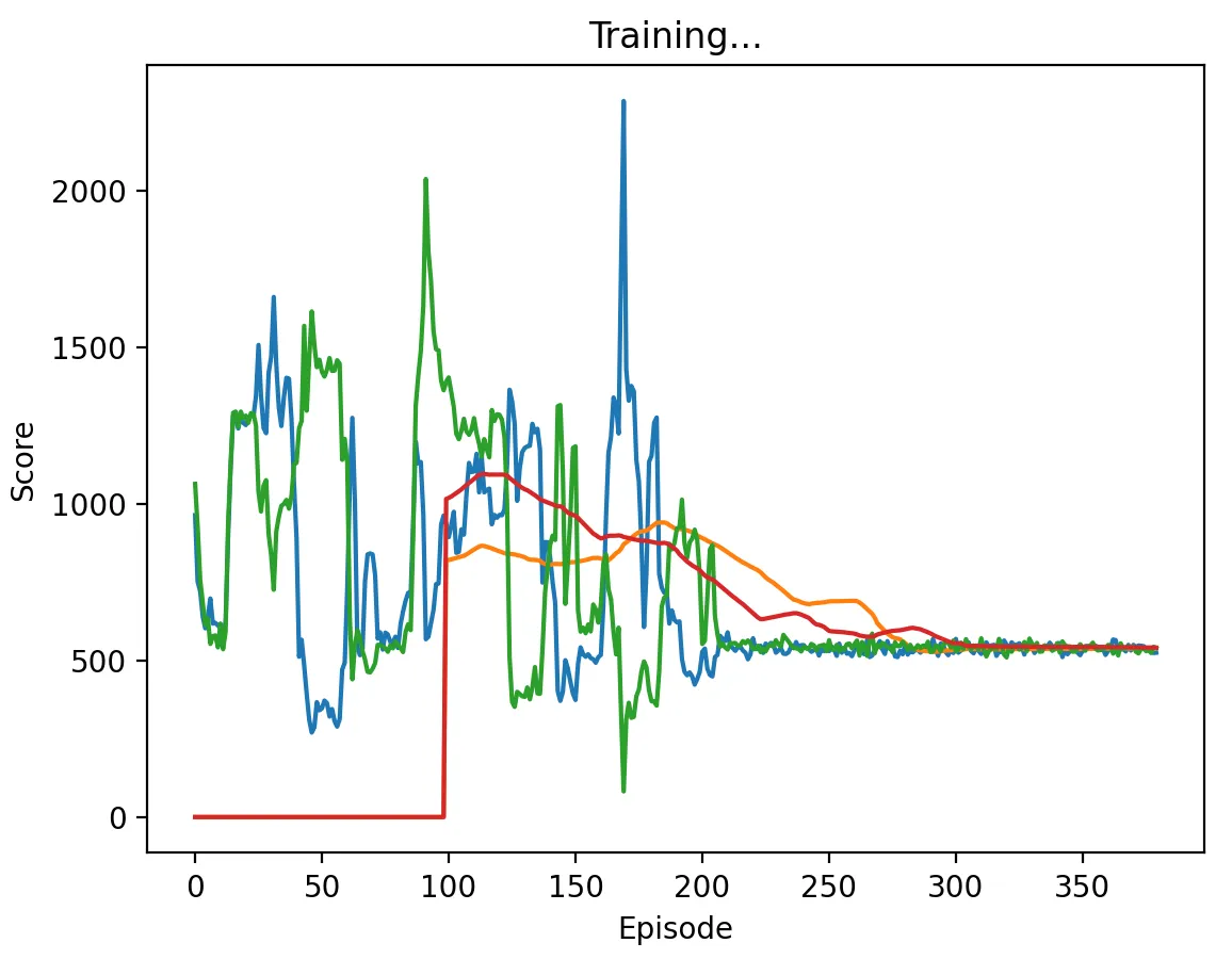 Figure 11: DQN Agent playing against another DQN agent with a high discount factor (0.95) and memory length 5. Interestingly, the agents took the longest to converge with this discount factor, converging to the (D,D) action profile only after about 200 episodes in multiple runs.
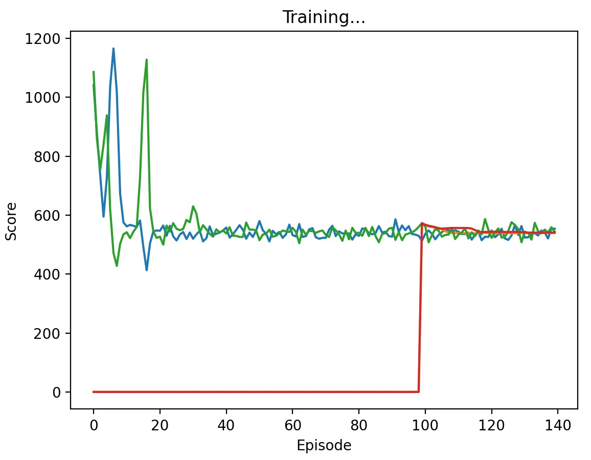 Figure 12: DQN Agent playing against another DQN agent with a high discount factor (1.0) and memory length 5. Agents converge much faster than when the discount factor was 0.95, taking about 20 episodes to do so. However, they converge to some mixed strategy that yields a score of about 550 per episode.
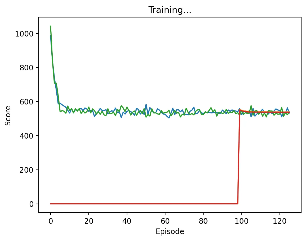 Figure 13: DQN Agent playing against another DQN agent with a low discount factor (0.1) and memory length 5. Agents converge much faster than when the discount factor was 0.95, taking about 5 episodes to do so. Again, they converge to some mixed strategy that yields a score of about 550 per episode.
Increases in memory length increased the speed of convergence, but did not significantly affect total scores.
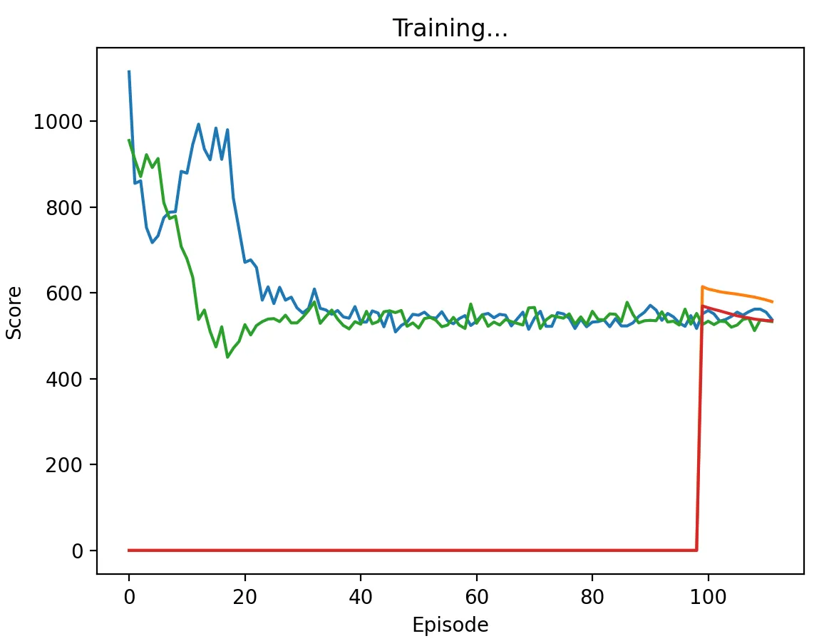 Figure 14: DQN Agent playing against another DQN agent with a high discount factor (0.95) and memory length 100. Agents converge much faster than when the memory was 5, taking about 35 episodes to do so.
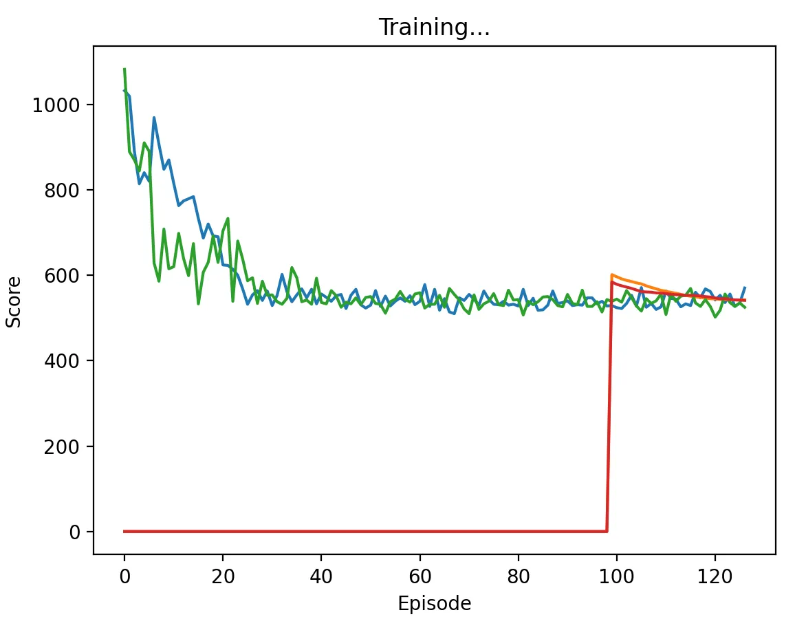 Figure 15: DQN Agent playing against another DQN agent with a high discount factor (0.95) and memory length 200. Agents converge much faster than when the memory was 5, taking about 35 episodes to do so. There was not an observable change in speed of convergence between a memory length of 100 and 200.
Chicken: Learning to Signal
Though our DQN agents had difficulty learning to cooperate in IPD, we were interested to see if they would learn to cooperate in a multiagent environment with correlated equilibria such as Chicken. Though our agents are trained using independent Q-networks, feedback from the environment still depends on the other agent. Hence, we tested our DQN agents to see if they learn to “signal” one another and are able to learn to play correlated equilibria, despite having independent learning networks.
The Game
We’ll assume the payoffs for Chicken are the following:
| W | G | |
|---|---|---|
| W | 0, 0 | 0, 2 |
| G | 2, 0 | -4, -4 |
And we note that the following action distributions are Nash equilibria of the game:
We run the same simulation with Chicken as with IPD, where each episode consists of 500 rounds, and we test our DQN agents against each other, with variances in .
Results
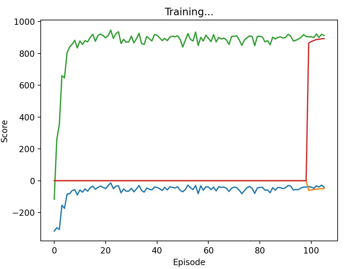 Figure 16a: DQN Agent playing against another DQN agent with a high discount factor (0.95) and memory length 5. Agents converge to Nash equilibrium relatively quickly, with one agent always playing W and another always playing G.
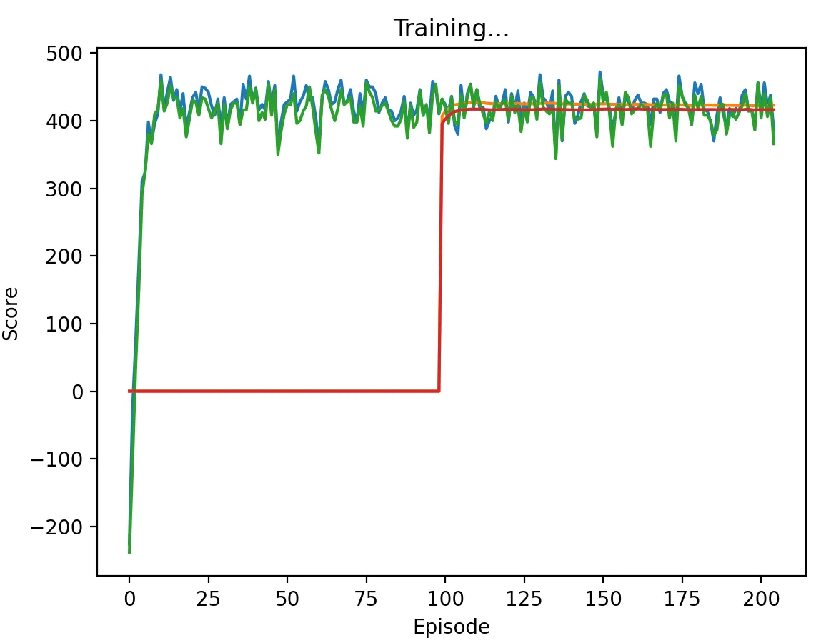 Figure 16b: DQN Agent playing against another DQN agent with a high discount factor (0.95) and memory length 5. Agents scores converge to about 400, i.e. they have an expected score of 4/5 per stage game. We thus find that they converge to a correlated equilibrium with action distribution:
The scoring scheme in Figure 16b arises with the same discount factor and memory length as in Figure 16a, though less frequently. Hence, we show that our agents are able to learn correlated equilibria, depending on the dynamics of the game in the initial episodes.
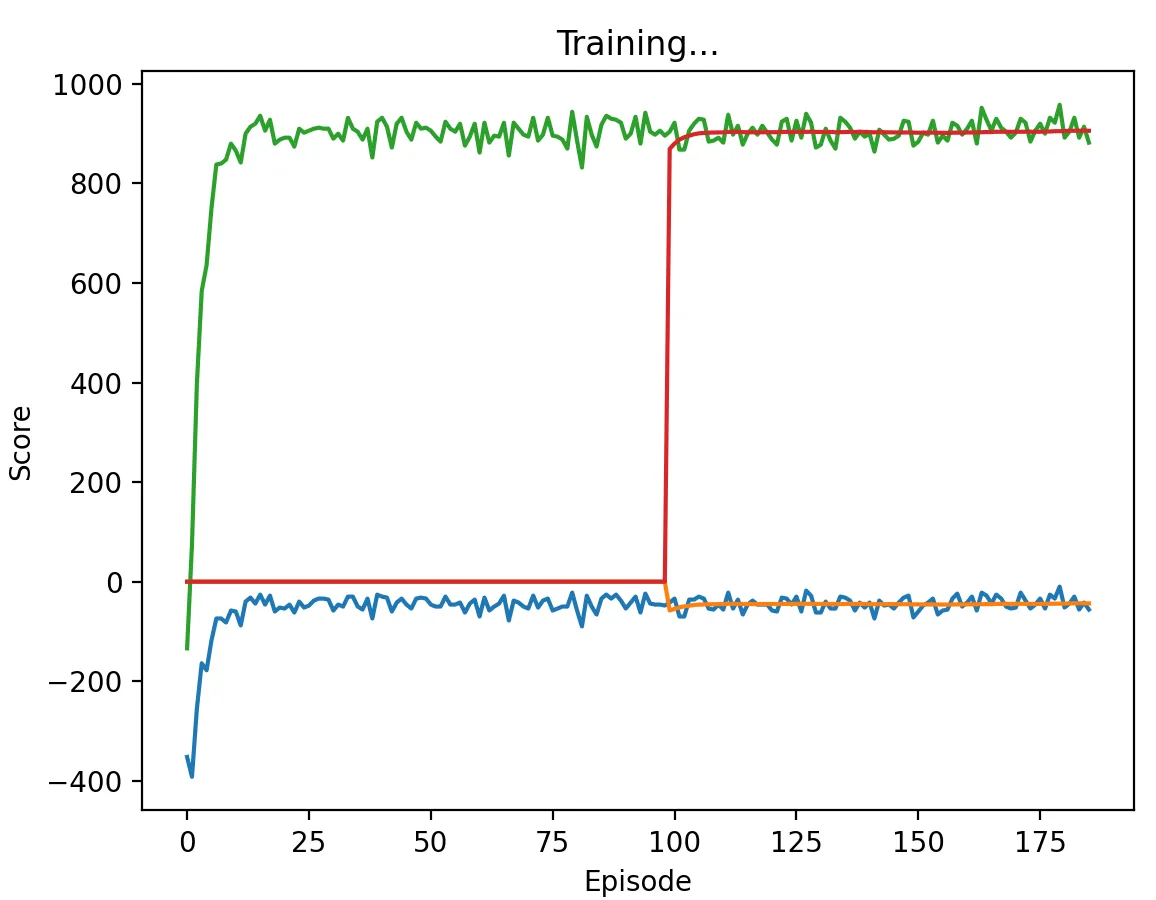 Figure 17a: DQN Agent playing against another DQN agent with a low discount factor (0.1) and memory length 5. Similarly to our high discount factor case, agents converge to Nash equilibrium relatively quickly, with one agent always playing W and another always playing G.
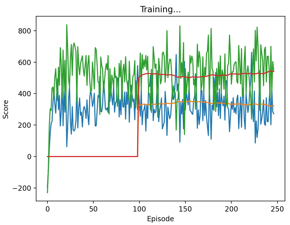 Figure 17b: DQN Agent playing against another DQN agent with a low discount factor (0.1) and memory length 5.
DQN agents with a low discount factor exhibit somewhat similar behavior to our high discount factor, converging to Nash Equilibria quickly in most cases, but similarly to our high discount factor case, we find that agents need not converge to repeated games of Pure Strategy Nash Equilibria. Furthermore, in this case, although the total scores of the agents with low discount factors have expected value 400 (similar to the agents with high discount factors), the variance in total scores in an episode is much greater.
Conclusions
Our exploration into RL has provided valuable insights into the challenges and opportunities presented by multi-agent environments, particularly when facing classic game-theoretic dilemmas such as the Prisoners’ Dilemma and the Game of Chicken. Much of the existing RL literature focuses on cooperative or competitive settings, yet the inherent duality of the Prisoners’ Dilemma introduces a unique complexity, where agents can dynamically shift between cooperation and competition.
By leveraging Deep Q-Learning (DQN), we successfully trained agents to engage with diverse strategies such as Tit-for-Tat (TFT), Random, and Pavlov. The exploration of scenarios with multiple DQN agents revealed intriguing dynamics. While the convergence of the Q-Learning algorithm is not guaranteed, our findings indicate that, over time, agents do converge to a total score.
Notably, in the Game of Chicken, in some cases our DQN agents displayed the ability to “signal” each other, deviating from strict Nash equilibrium strategies, though these emerged more often (either (W,G) or (G,W) being played at every stage game). The emergence of correlated equilibria in certain scenarios resulted in total scores that favored both agents, showcasing the potential for nuanced cooperation beyond traditional equilibrium outcomes.
In summary, our research not only advances our understanding of RL in multi-agent environments but also underscores the adaptability and emergent behaviors achievable through DQN. The interplay between cooperation and competition, coupled with the ability to signal and discover correlated equilibria, opens exciting avenues for future research in multi-agent reinforcement learning and its applications in complex decision-making scenarios.
Acknowledgements
This research was originally presented as the final project for the CS 136 Economics and Computation course taught at Harvard University in the Fall of 2023 by Professor David C. Parkes.
References
-
Tampuu, A., Matiisen, T., Kodelja, D., Kuzovkin, I., Korjus, K., Aru, J., Aru, J., & Vicente, R. (2015). Multiagent Cooperation and Competition with Deep Reinforcement Learning. arXiv:1511.08779
-
Terry, J. K., Black, B., Grammel, N., Jayakumar, M., Hari, A., Sullivan, R., Santos, L., Perez, R., Horsch, C., Dieffendahl, C., Williams, N. L., Lokesh, Y., & Ravi, P. (2021). PettingZoo: Gym for Multi-Agent Reinforcement Learning. arXiv:2009.14471
-
Sen, S., Sekaran, M., & Hale, J. (1994). Learning to Coordinate without Sharing Information. Proceedings of AAAI-94, 426-431.
-
Sutton, R. S., & Barto, A. G. (2018). Reinforcement learning: An introduction (2nd ed.). The MIT Press.
-
Sandholm, T. W., & Crites, R. H. (1996). Multiagent reinforcement learning in the Iterated Prisoner’s Dilemma. Biosystems, 37(1–2), 147-166. https://doi.org/10.1016/0303-2647(95)01551-5
-
Shoham, Y., Powers, R., & Grenager, T. (2007). If multi-agent learning is the answer, what is the question? Artificial Intelligence, 171(7), 365-377. https://doi.org/10.1016/j.artint.2006.02.006